If you have any issues with one of the packages hosted in this repository, please feel free to open an issue (preferred instead of using Contact Maintainers on chocolatey.org).
This repository contains chocolatey automatic packages.
The repository is setup so that you can manage your packages entirely from the GitHub web interface (using AppVeyor to update and push packages) and/or using the local repository copy.
In a package directory run: Test-Package. This function can be used to start testing in chocolatey-test-environment via Vagrant parameter or it can test packages locally.
Automatic package update
Single package
Run from within the directory of the package to update that package:
cd <package_dir>
./update.ps1
If this script is missing, the package is not automatic.
Set $au_Force = $true prior to script call to update the package even if no new version is found.
Multiple packages
To update all packages run ./update_all.ps1. It accepts few options:
./update_all.ps1 -Name a*# Update all packages which name start with letter 'a'
./update_all.ps1 -ForcedPackages 'cpu-z copyq'# Update all packages and force cpu-z and copyq
./update_all.ps1 -ForcedPackages 'copyq:1.2.3'# Update all packages but force copyq with explicit version
./update_all.ps1 -Root 'c:\packages'# Update all packages in the c:\packages folder
The following global variables influence the execution of update_all.ps1 script if set prior to the call:
$au_NoPlugins=$true#Do not execute plugins$au_Push=$false#Do not push to chocolatey
You can also call AU method Update-AUPackages (alias updateall) on its own in the repository root. This will just run the updater for the each package without any other option from update_all.ps1 script. For example to force update of all packages with a single command execute:
updateall -Options ([ordered]@{ Force = $true })
Pushing To Community Repository Via Commit Message
You can force package update and push using git commit message. AppVeyor build is set up to pass arguments from the commit message to the ./update_all.ps1 script.
If commit message includes [AU <forced_packages>] message on the first line, the forced_packages string will be sent to the updater.
Examples:
[AU pkg1 pkg2]
Force update ONLY packages pkg1 and pkg2.
[AU pkg1:ver1 pkg2 non_existent]
Force pkg1 and use explicit version ver1, force pkg2 and ignore non_existent.
To see how versions behave when package update is forced see the force documentation.
You can also push manual packages with command [PUSH pkg1 ... pkgN]. This works for any package anywhere in the file hierarchy and will not invoke AU updater at all.
If there are no changes in the repository use --allow-empty git parameter:
Way1 Extract download zip on wp-content/plugins/wpsf-framework folder under your plugin directory
Way2 Upload zip file from wordpess plugins panel -> add new -> upload plugin
Active WPSF Framework plugin from wordpress plugins panel
Yay! Right now you are ready to configure framework, metaboxes, taxonomies, wp customize, shortcoder
Take a look for config files from wp-content/plugins/wpsf-framework/config folder also you can manage config files from theme directory. see overriding files method.
You can override an existing file without change themename/wpsf-framework folder. just create one themename/wpsf-framework-override folder on your theme directory. for eg:
Simulated Hospital is a tool that generates realistic and configurable
hospital patient data in
HL7v2 format.
Disclaimer: This is not an officially supported Google product.
Overview
A hospital’s Electronic Health Record (EHR) system contains patients’ health
information. EHRs use messages to communicate clinical actions like the
admission of a patient, ordering a blood test, or getting test results. This
flow of messages describes the lifetime of a patient’s stay in a hospital.
Most EHRs use a message format called
HL7v2,
which is ugly and tedious to type. Simulated Hospital generates messages in
HL7v2 format from sequences of clinical actions. The generated HL7v2 messages
can be sent to an
MLLP
host, saved to a txt file, or printed to the console.
Simulated Hospital helps developers build and test clinical apps without access
to real data. It makes it easy to generate HL7v2 messages that reproduce
realistic situations in clinical settings.
Basic Concepts
The basic behavior of Simulated Hospital can be summarized as follows:
Simulated Hospital creates patients at a configurable rate.
When Simulated Hospital creates a patient, it associates the patient with a
pathway.
A pathway models the events that will occur to the patient.
Simulated Hospital runs events when they are due, in real time.
When events run, they generate HL7v2 messages.
Pathways
A pathway is a sequence of clinical actions or events that describe the lifetime
of a patient’s stay in a hospital. An example of a simple pathway could be: the
patient is admitted, a doctor orders an X-ray, the X-ray is taken, and the
patient is discharged. Each action typically generates one or more HL7v2
messages.
Simulated Hospital runs pathways. You can configure Simulated Hospital to run
the pathways that you want, including how frequently to run each one. The
application includes a few built-in pathways (see the folder
“config/pathways”) but most people will want to write their own.
Pathways are written using YAML or JSON and are human readable. The events are
defined with words that are common in clinical settings such as “admission”,
“discharge”, etc., and utility actions such as time delays.
Write pathways to create patients with specific
conditions, for instance, a patient with appendicitis that has sets of Vital
Signs taken periodically.
Change the default behavior of Simulated Hospital using
command-line arguments, including:
What pathways Simulated Hospital runs and their distribution, i.e., what
pathways should run more frequently than others.
What specific values to set for some fields in the HL7v2 messages in
order to comply, or not, with the values in the HL7v2 standard. For
instance, you can configure what should be set as the Sending Facility
in the generated messages, or what keyword to use to represent that a
set of laboratory results is amended.
The demographics of the patients that are generated: names, surnames,
ethnicity, etc. For instance, you can configure how many patients will
have middle names, or what is the probability that a patient will have
pre-existing allergies.
Control a running instance Simulated Hospital using its
Dashboard(screenshot).
Using the dashboard, you can do the following:
Change the message-sending rate of a self-running simulation.
Start an ad-hoc pathway or send an HL7v2 message.
Extend Simulated Hospital with advanced functionality
using source code. For instance, you can change the format of the
identifiers that Simulated Hospital generates, or create your own behavior
for some events.
Compares Population Density Estimates and Satellite Night Light Mesurements
Presentation
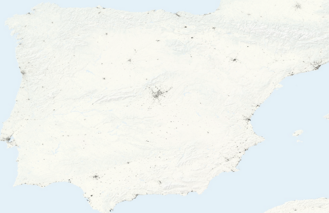
This repository compares estimates of population density and satellite measurements of night light.
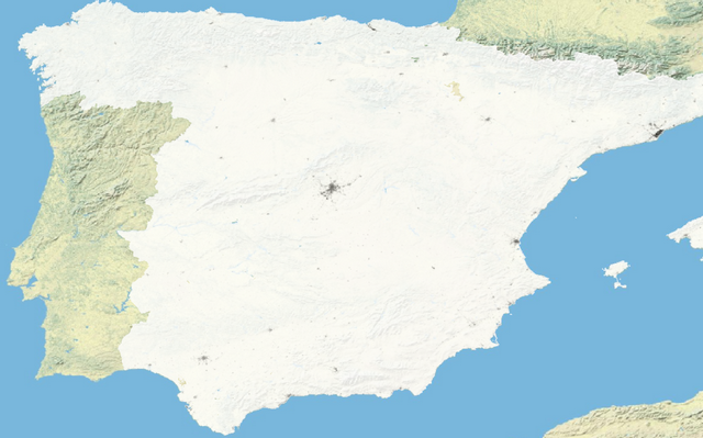
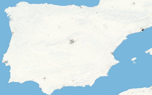
It is applied with data for Spain (for simplicity, exclusing Canary Islands), but it can easily be used for different datasets.
Data
The sources for the population density datasets are:
2 WorldPop, UN adjusted, unconstrained, 2020, 1 km resolution, which provides population counts and is procesed with the script CALC DENS POP to obtain the required population density raster.
3 DMSP-OLS, for 2010, averaged with radiance calibration.
All raster files have been clipped to (-9.65, 43.9; 4.5, 36.0) deg (lon, lat).
The rasters are, at plain sight, correct as shown in the following snapshots from QGIS with a transparency of 80%:
Internal correlations
The datasets have been compared within each type of data, with the following main results.
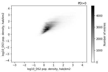
Population Density
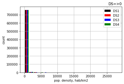
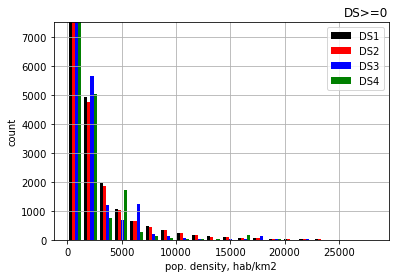
The datasets are highly correlated by pairs 1-2 and 3-4, as should be expected, and only moderately correlated across these groups as indicated by the Pearson coefficients (after removing the no-data, maintaining the 0s):
DS1-2 = 0.995.
DS1-3 = 0.693.
DS1-4 = 0.693.
DS2-3 = 0.681.
DS2-4 = 0.681.
DS3-4 = 1.000.
The histograms are controlled by the low densities:
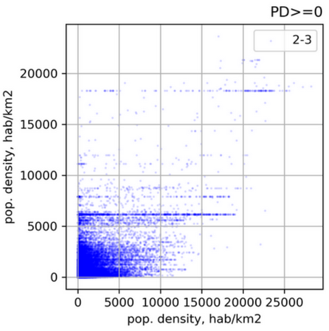
The bivariate graphs confirm the moderate correlation:
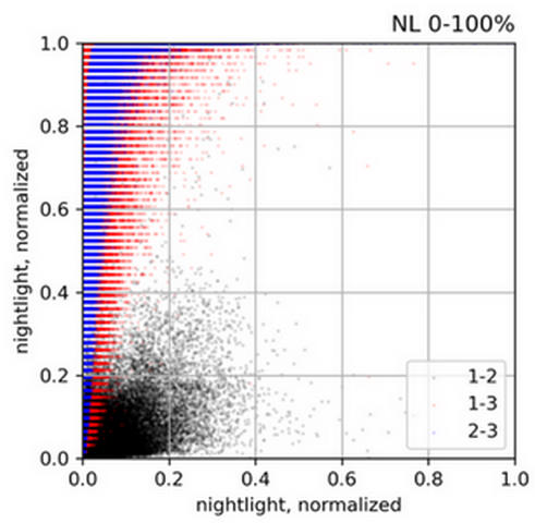
Nightlight Measurements
The correlation among the datasets is also just moderate, as indicated by the Pearson coefficients (after removing the 0s and no-data):
DS1-2 = 0.632.
DS1-3 = 0.507.
DS2-3 = 0.646.
Normalizing the data yields a loose relationship:
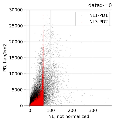
External correlations
The rather low internal correlations among the datasets raises the question of which can actually be the strength of the relationship between population density and night-light measurements, and whether the selection of the appropriate pair of datasets (population density, night-light measurement) becomes a sort of data bazaar.
The results of the bivariate correlations, measured by the Pearson coefficient, are:
NL1-PD1 = 0.773.
NL1-PD2 = 0.763.
NL1-PD3 = 0.560.
NL1-PD4 = 0.559.
NL2-PD1 = 0.732.
NL2-PD2 = 0.732.
NL2-PD3 = 0.649.
NL2-PD4 = 0.638.
NL3-PD1 = 0.447.
NL3-PD2 = 0.438.
NL3-PD3 = 0.443.
NL3-PD4 = 0.441.
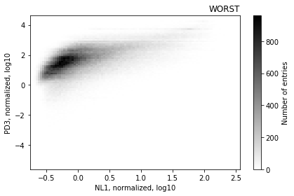
The scatter plot for best and worst correlations is:
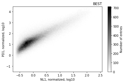
The results improve with a log-log transformation:
NL1-PD1 = 0.875.
NL1-PD2 = 0.872.
NL1-PD3 = 0.570.
NL1-PD4 = 0.571.
NL2-PD1 = 0.765.
NL2-PD2 = 0.762.
NL2-PD3 = 0.587.
NL2-PD4 = 0.588.
NL3-PD1 = 0.829.
NL3-PD2 = 0.827.
NL3-PD3 = 0.597.
NL3-PD4 = 0.600.
And the corresponding heatmaps for the best and worst log-log correlations are:
Scripts
Three scripts are provided:
POP CHECK, performs the calculations with the population density rasters.
NL CHECK, which does a similar task with the nightlight measurements.
NL-POP CROSS, which compares the nightlight measurements to the population density estimates.
The scripts are written in Python. They use the library rasterio, which I have not been able to run under python 3.8, but it works well under python 3.6.
They have been uploaded as they are on my computer: modifying the location of the files and other preferences should be quite straightforward.
Identifying key traits in Hawaiian fish to predict risk of extinction
EDS 222 Statistics for Environmental Data Science Final Project
Summary
This is the original code repository for the following blog post and my final project for a statistics course at the Bren School of Envrionmental Science and Management taught by Tamma Carleton (completed in early December 2022). I investigate Hawaiian fish ecological traits – such as size, endemism, and reef-association – to find their probability of being threatened as ranked by the IUCN Red List.
Global human activity threatens many species with extinction. According to the International Union and Conservation of Nature (IUCN), “More than 41,000 species are threatened with extinction. That is still 28% of all assessed species.” [1]. Increased extinction and loss of biodiversity can have severe ecological, economic, and cultural impacts. Cardinale et al.’s deep dive into biodiversity and ecosystem services research conclude that biodiversity loss reduces ecological communities’ efficiency, stability, and productivity. Decreased productivity from ecosystem services can have a negative impact on ecosystem economics [2]. Additionally, cultures worldwide have strong ties to local flora and fauna, much of which now face extinction risk. Improving understanding of extinction risk is ecologically, economically, and culturally important.
Wildlife scientists have been working to understand what ecological traits of vertebrates predict threat level, and what common risk factors drive those threat level rates. Munstermann et al. investigate what terrestrial vertebrate functional groups are most at risk of extinction threat and find that cave dwelling amphibian, arboreal quadrupedal mammals, aerial and scavenging birds, and pedal squamates are at high risk [3]. This knowledge can help inform policies and practices with the goal to decrease threats of extinction of wildlife. However, less comprehensive research has been done to conduct similar analyses on marine species.
In recent years, the waters surrounding the Hawaiian Islands have been exposed to ecological changes due to mass coral bleaching events, El Niño events, and pollution. Rapidly changing marine ecosystems may pose a threat to Hawaiian fish. Fish hold significant cultural value in Hawaiʻi, and many local people rely on seafood as a major source of protein. However, approximately 72% of fish in Hawaiʻi present in FishBase have been evaluated by the IUCN and have sufficient data to be assessed. Here I run a small-scale analysis to investigate Hawaiian fish ecological traits – such as endemism, size, and reef-association – to predict a binary status on the IUCN red list and predict which unevaluated fish species in Hawaiʻi may be threatened.
Data
For my analyses I use the IUCN Red List data accessed via the IUCN Red List API[1] and package rredlist[4]. Fish ecological data were accessed from FishBase.[5] via package rfishbase[6].
All References
[1] “IUCN,” IUCN Red List of Threatened Species. Version 2022-1, 2022. https://www.iucnredlist.org/ (accessed Dec. 02, 2022).
[2] B. J. Cardinale et al., “Biodiversity loss and its impact on humanity,” Nature, vol. 486, no. 7401, Art. no. 7401, Jun. 2012, doi: 10.1038/nature11148.
[3] M. J. Munstermann et al., “A global ecological signal of extinction risk in terrestrial vertebrates,” Conserv. Biol., vol. 36, no. 3, p. e13852, 2022, doi: 10.1111/cobi.13852.
[4] “IUCN,” IUCN Red List of Threatened Species. Version 2022-1, 2015. www.iucnredlist.org
[6] C. Boettiger, D. Temple Lang, and P. Wainwright, “rfishbase: exploring, manipulating and visualizing FishBase data from R.,” J. Fish Biol., 2012, doi: https://doi.org/10.1111/j.1095-8649.2012.03464.x.
[7] W. J. Ripple, C. Wolf, T. M. Newsome, M. Hoffmann, A. J. Wirsing, and D. J. McCauley, “Extinction risk is most acute for the world’s largest and smallest vertebrates,” Proc. Natl. Acad. Sci. U. S. A., vol. 114, no. 40, pp. 10678–10683, Oct. 2017, doi: 10.1073/pnas.1702078114.
[8] K. D. Bahr, P. L. Jokiel, and K. S. Rodgers, “The 2014 coral bleaching and freshwater flood events in Kāneʻohe Bay, Hawaiʻi,” PeerJ, vol. 3, p. e1136, Aug. 2015, doi: 10.7717/peerj.1136.
Create a terraform.tfvars file in the root of this project with metal_api_token and project_id defined. These are the required variables needed to run terraform apply. See variables.tf for additional settings that you may wish to customize.
# terraform.fvarsmetal_api_token="...your Metal User API Token here..."project_id="...your Metal Project API Token here..."
Note
Project API Tokens can not be used to access some Gateway features used by this project. A User API Token is required.
Terraform will create an Equinix Metal VLAN, Metal Gateway, IP Reservation, and Equinix Metal servers to act as the EKS-A Admin node and worker devices. Terraform will also create the initial hardware.csv with the details of each server and register this with the eks-anywhere CLI to create the cluster. The worker nodes will be provisioned through Tinkerbell to act as a control-plane node and a worker-node.
root@eksa-admin:~# kubectl get nodes
NAME               STATUS   ROLES                  AGE     VERSION
eksa-node-cp-001   Ready    control-plane,master   7m56s   v1.22.10-eks-7dc61e8
eksa-node-worker-001   Ready    <none>                 5m30s   v1.22.10-eks-7dc61e8
How to expand a cluster
This section is an example of adding a new node of the exact same time as the previous nodes to the cluster. For example, if you use project defaults you’ll want to add a m3.small.x86 as the new node. Also, this example is just adding a new worker node for simplicity. Adding control plane nodes is possible, but requires thinking through how many nodes are added as well as labeling them as type=cp instead of type=worker.
Deploy an additional node
NEW_HOSTNAME="your new hostname"
POOL_ADMIN="IP address of your admin machine"
metal device create --plan m3.small.x86 --metro da --hostname $NEW_HOSTNAME
--ipxe-script-url http://$POOL_ADMIN/ipxe/ --operating-system custom_ipxe
Make note of the device’s UUID, maybe use metal device get to list them.
(Optional) Connect the cluster to EKS with EKS Connector
This section covers the basic steps to connect your cluster to EKS with the EKS Connector. There are many more details (include pre-requisites like IAM permissions) in the EKS Connector Documentation.
If it succeeded, the output will show several .yaml files that were created and need to be registered with the cluster. For example, at the time of writing, applying those files would be done like so:
Note
This section will serve as manual instructions for installing EKS-A Bare Metal on Equinix Metal. The Terraform install above performs all of these steps for you.
These instructions offer a step-by-step install with copy+paste commands that simplify the process. Refer to the open issues and please open issues if you encounter something not represented there.
Steps below align with EKS-A on Bare Metal instructions. While the steps below are intended to be complete, follow along with the EKS-A Install guide for best results.
Steps to run locally and in the Equinix Metal Console
Create an EKS-A Admin machine:
Using the metal-cli:
Create an API Key and register it with the Metal CLI:
metal init
metal device create --plan=m3.small.x86 --metro=da --hostname eksa-admin --operating-system ubuntu_20_04
Create a VLAN:
metal vlan create --metro da --description eks-anywhere --vxlan 1000
Create a Public IP Reservation (16 addresses):
metal ip request --metro da --type public_ipv4 --quantity 16 --tags eksa
These variables will be referred to in later steps in executable snippets to refer to specific addresses within the pool. The correct IP reservation is chosen by looking for and expecting a single IP reservation to have the “eksa” tag applied.
#Capture the ID, Network, Gateway, and Netmask using jq
VLAN_ID=$(metal vlan list -o json | jq -r '.virtual_networks | .[] | select(.vxlan == 1000) | .id')
POOL_ID=$(metal ip list -o json | jq -r '.[] | select(.tags | contains(["eksa"]))? | .id')
POOL_NW=$(metal ip list -o json | jq -r '.[] | select(.tags | contains(["eksa"]))? | .network')
POOL_GW=$(metal ip list -o json | jq -r '.[] | select(.tags | contains(["eksa"]))? | .gateway')
POOL_NM=$(metal ip list -o json | jq -r '.[] | select(.tags | contains(["eksa"]))? | .netmask')# POOL_ADMIN will be assigned to eksa-admin within the VLAN
POOL_ADMIN=$(python3 -c 'import ipaddress; print(str(ipaddress.IPv4Address("'${POOL_GW}'")+1))')# PUB_ADMIN is the provisioned IPv4 public address of eks-admin which we can use with ssh
PUB_ADMIN=$(metal devices list -o json | jq -r '.[] | select(.hostname=="eksa-admin") | .ip_addresses [] | select(contains({"public":true,"address_family":4})) | .address')# PORT_ADMIN is the bond0 port of the eks-admin machine
PORT_ADMIN=$(metal devices list -o json | jq -r '.[] | select(.hostname=="eksa-admin") | .network_ports [] | select(.name == "bond0") | .id')# POOL_VIP is the floating IPv4 public address assigned to the current lead kubernetes control plane
POOL_VIP=$(python3 -c 'import ipaddress; print(str(ipaddress.ip_network("'${POOL_NW}'/'${POOL_NM}'").broadcast_address-1))')
TINK_VIP=$(python3 -c 'import ipaddress; print(str(ipaddress.ip_network("'${POOL_NW}'/'${POOL_NM}'").broadcast_address-2))')
Create a Metal Gateway
metal gateway create --ip-reservation-id $POOL_ID --virtual-network $VLAN_ID
Create Tinkerbell worker nodes eksa-node-001 – eksa-node-002 with Custom IPXE http://{eks-a-public-address}. These nodes will be provisioned as EKS-A Control Plane OR Worker nodes.
forain {1..2};do
metal device create --plan m3.small.x86 --metro da --hostname eksa-node-00$a \
--ipxe-script-url http://$POOL_ADMIN/ipxe/ --operating-system custom_ipxe
done
Note that the ipxe-script-url doesn’t actually get used in this process, we’re just setting it as it’s a requirement for using the custom_ipxe operating system type.
Add the vlan to the eks-admin bond0 port:
metal port vlan -i $PORT_ADMIN -a $VLAN_ID
Configure the layer 2 vlan network on eks-admin with this snippet:
ssh root@$PUB_ADMIN tee -a /etc/network/interfaces <<EOSauto bond0.1000iface bond0.1000 inet static pre-up sleep 5 address $POOL_ADMIN netmask $POOL_NM vlan-raw-device bond0EOS
Activate the layer 2 vlan network with this command:
ssh root@$PUB_ADMIN systemctl restart networking
Convert eksa-node-* ‘s network ports to Layer2-Unbonded and attach to the VLAN.
node_ids=$(metal devices list -o json | jq -r '.[] | select(.hostname | startswith("eksa-node")) | .id')
i=1 # We will increment "i" for the eksa-node-* nodes. "1" represents the eksa-admin node.foridin$(echo $node_ids);dolet i++
BOND0_PORT=$(metal devices get -i $id -o json | jq -r '.network_ports [] | select(.name == "bond0") | .id')
ETH0_PORT=$(metal devices get -i $id -o json | jq -r '.network_ports [] | select(.name == "eth0") | .id')
metal port convert -i $BOND0_PORT --layer2 --bonded=false --force
metal port vlan -i $ETH0_PORT -a $VLAN_IDdone
Capture the MAC Addresses and create hardware.csv file on eks-admin in /root/ (run this on the host with metal cli on it):
Use metal and jq to grab HW MAC addresses and add them to the hardware.csv:
node_ids=$(metal devices list -o json | jq -r '.[] | select(.hostname | startswith("eksa-node")) | .id')
i=1 # We will increment "i" for the eksa-node-* nodes. "1" represents the eksa-admin node.foridin$(echo $node_ids);do# Configure only the first node as a control-panel nodeif [ "$i"= 1 ];then TYPE=cp;else TYPE=worker;fi;# change to 3 for HA
NODENAME="eks-node-00$i"let i++
MAC=$(metal device get -i $id -o json | jq -r '.network_ports | .[] | select(.name == "eth0") | .data.mac')
IP=$(python3 -c 'import ipaddress; print(str(ipaddress.IPv4Address("'${POOL_GW}'")+'$i'))')echo"$NODENAME,Equinix,${MAC},${IP},${POOL_GW},${POOL_NM},8.8.8.8|8.8.4.4,/dev/sda,type=${TYPE}">> hardware.csv
done
The BMC fields are omitted because Equinix Metal does not expose the BMC of nodes. EKS Anywhere will skip BMC steps with this configuration.
Copy hardware.csv to eksa-admin:
scp hardware.csv root@$PUB_ADMIN:/root
We’ve now provided the eksa-admin machine with all of the variables and configuration needed in preparation.
Steps to run on eksa-admin
Login to eksa-admin with the LC_POOL_ADMIN and LC_POOL_VIP variable defined
# SSH into eksa-admin. The special args and environment setting are just tricks to plumb $POOL_ADMIN and $POOL_VIP into the eksa-admin environment.
LC_POOL_ADMIN=$POOL_ADMIN LC_POOL_VIP=$POOL_VIP LC_TINK_VIP=$TINK_VIP ssh -o SendEnv=LC_POOL_ADMIN,LC_POOL_VIP,LC_TINK_VIP root@$PUB_ADMIN
Note
The remaining steps assume you have logged into eksa-admin with the SSH command shown above.
Append the following to the $CLUSTER_NAME.yaml file.
cat << EOF >> $CLUSTER_NAME.yaml
---
apiVersion: anywhere.eks.amazonaws.com/v1alpha1kind: TinkerbellTemplateConfigmetadata:
name: ${CLUSTER_NAME}spec:
template:
global_timeout: 6000id: ""name: ${CLUSTER_NAME}tasks:
- actions:
- environment:
COMPRESSED: "true"DEST_DISK: /dev/sdaIMG_URL: https://anywhere-assets.eks.amazonaws.com/releases/bundles/29/artifacts/raw/1-25/bottlerocket-v1.25.6-eks-d-1-25-7-eks-a-29-amd64.img.gzimage: public.ecr.aws/eks-anywhere/tinkerbell/hub/image2disk:6c0f0d437bde2c836d90b000312c8b25fa1b65e1-eks-a-29name: stream-imagetimeout: 600
- environment:
CONTENTS: | # Version is required, it will change as we support # additional settings version = 1 # "eno1" is the interface name # Users may turn on dhcp4 and dhcp6 via boolean [enp1s0f0np0] dhcp4 = true dhcp6 = false # Define this interface as the "primary" interface # for the system. This IP is what kubelet will use # as the node IP. If none of the interfaces has # "primary" set, we choose the first interface in # the file primary = trueDEST_DISK: /dev/sda12DEST_PATH: /net.tomlDIRMODE: "0755"FS_TYPE: ext4GID: "0"MODE: "0644"UID: "0"image: public.ecr.aws/eks-anywhere/tinkerbell/hub/writefile:6c0f0d437bde2c836d90b000312c8b25fa1b65e1-eks-a-29name: write-netplanpid: hosttimeout: 90
- environment:
BOOTCONFIG_CONTENTS: | kernel { console = "ttyS1,115200n8" }DEST_DISK: /dev/sda12DEST_PATH: /bootconfig.dataDIRMODE: "0700"FS_TYPE: ext4GID: "0"MODE: "0644"UID: "0"image: public.ecr.aws/eks-anywhere/tinkerbell/hub/writefile:6c0f0d437bde2c836d90b000312c8b25fa1b65e1-eks-a-29name: write-bootconfigpid: hosttimeout: 90
- environment:
DEST_DISK: /dev/sda12DEST_PATH: /user-data.tomlDIRMODE: "0700"FS_TYPE: ext4GID: "0"HEGEL_URLS: http://${LC_POOL_ADMIN}:50061,http://${LC_TINK_VIP}:50061MODE: "0644"UID: "0"image: public.ecr.aws/eks-anywhere/tinkerbell/hub/writefile:6c0f0d437bde2c836d90b000312c8b25fa1b65e1-eks-a-29name: write-user-datapid: hosttimeout: 90
- image: public.ecr.aws/eks-anywhere/tinkerbell/hub/reboot:6c0f0d437bde2c836d90b000312c8b25fa1b65e1-eks-a-29name: reboot-imagepid: hosttimeout: 90volumes:
- /worker:/workername: ${CLUSTER_NAME}volumes:
- /dev:/dev
- /dev/console:/dev/console
- /lib/firmware:/lib/firmware:roworker: '{{.device_1}}'version: "0.1"EOF
Create an EKS-A Cluster. Double check and be sure $LC_POOL_ADMIN and $CLUSTER_NAME are set correctly before running this (they were passed through SSH or otherwise defined in previous steps). Otherwise manually set them!
Steps to run locally while eksctl anywhere is creating the cluster
When the command above indicates that it is Creating new workload cluster, reboot the two nodes. This
is to force them attempt to iPXE boot from the tinkerbell stack that eksctl anywhere command creates.
Note that this must be done without interrupting the eksctl anywhere create cluster command.
Option 1 – You can use this command to automate it, but you’ll need to be back on the original host.
Option 2 – Instead of rebooting the nodes from the host you can force the iPXE boot from your local by
accessing each node’s SOS console.
You can retrieve the uuid and facility code of each node using the metal cli, UI Console or the Equinix Metal’s API.
By default, any existing ssh key in the project can be used to login.
You can see the below logs message if the whole process is successful.
Installing networking on workload cluster
Creating EKS-A namespace
Installing cluster-api providers on workload cluster
Installing EKS-A secrets on workload cluster
Installing resources on management cluster
Moving cluster management from bootstrap to workload cluster
Installing EKS-A custom components (CRD and controller) on workload cluster
Installing EKS-D components on workload cluster
Creating EKS-A CRDs instances on workload cluster
Installing GitOps Toolkit on workload cluster
GitOps field not specified, bootstrap flux skipped
Writing cluster config file
Deleting bootstrap cluster
:tada: Cluster created!
--------------------------------------------------------------------------------------
The Amazon EKS Anywhere Curated Packages are only available to customers with the
Amazon EKS Anywhere Enterprise Subscription
--------------------------------------------------------------------------------------
Enabling curated packages on the cluster
Installing helm chart on cluster	{"chart": "eks-anywhere-packages", "version": "0.2.30-eks-a-29"}
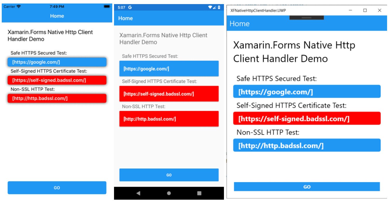
Instead of using the .NET managed HttpClientHandler, we need make sure to use the Native Client Handlers of each platform with our HttpClient, for the sake of performance, smaller executables, and security advantage.
AndroidClientHandler
-AndroidClientHandler is the new handler that delegates to native Java code and Android OS instead of implementing everything in managed code. This option has better performance and smaller executable size.
NSUrlSessionHandler
-The NSURLSession-based handler is based on the native NSURLSession framework available in iOS 7 and newer. This options has better performance and smaller executable size, supports TLS 1.2 standard.
WinHttpHandler
-WinHttpHandler is implemented as a thin wrapper on the WinHTTP interface of Windows and is only supported on Windows systems. Provides developers with more granular control over the application’s HTTP communication than the default HttpClientHandler class.
TempLogger reads temperature from a sensor attached to an Arduino board. It writes it into
an SQLite database. Temperature history can be viewed in a simple web application.
How to use
Setting up Arduino
Compile and upload the code from ./src/temperature.ino to your Arduino board in Arduino IDE.
The code is designed to work with the TMP36 temperature sensor and input voltage of 5V. The sensor
output should be attached to the A0 pin. Arduino writes the temperature to the serial port.
Python environment
In this project I use Rye package manager. After installing it you can run
$ rye sync
to create a virtual environment for the project.
Logger
Logger is responsible for reading the temperature from a serial port and storing it in a database.
You can start it like this:
$ rye run src/temp_logger/logger.py {path-to-serial-port} {path-to-database}
On Ubuntu 22.04 and Fedora 38, the serial port path was /dev/ttyACM0. Make sure that you
can read data from this device. On both Ubuntu and Fedora I achieved this by adding the user
to the dialup group.
Web interface
You can start the web interface like this:
$ rye run src/temp_logger/web.py
This will start the web interface showing a temperature graph at port 5000.
I use Quart – an async version of Flask to implement the
web interface.


![imgbot[bot]](http://thebios.top/wp-content/uploads/2025/08/4706)


 https://github.com/AdmiringWorm/chocolatey-packages
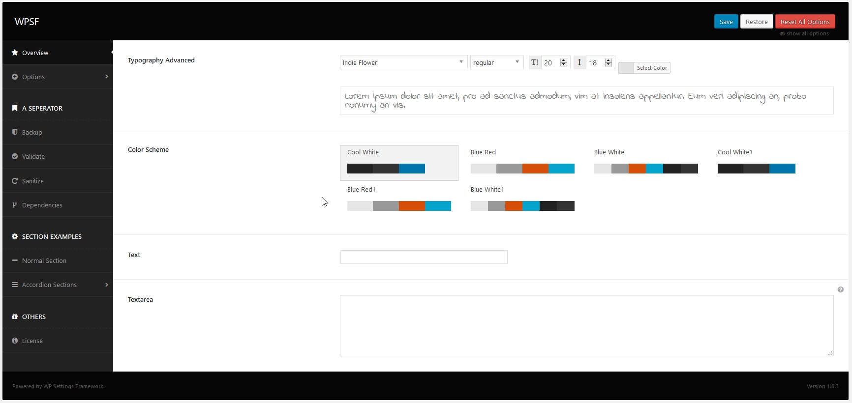


